This note is inspired by several time-nuts [1] postings. Doug Hogarth writes:
I once analyzed my 5065A and said it seemed aging slightly worse than spec (for example 1.23e-11/month). But that is old and I can't remember the detail.
So I just loaded up data file where I had two months days of continuous 5065A run against my 5071A-001 (high perf cesium). I remove the first day because Rb was definite warming up, and a couple more days because I think it was still not quite stable. Also there was a couple hundred nanosecond jump around the 18th day so perhaps that should be adjusted (but I left it as-is for this run).
Stable32 quadratic drift analysis says a=9.1e-5, b=-6.75e-11, c=-4.04e-17, slope=-8.09e-18
Put another way, if you remove linear frequency offset, the resulting phase parabola goes up from around -1.9usec to .9usec and then back down to -1.9usec (over the two months). If you remove the quadratic drift, the range is +/- couple hundred nanoseconds (but the jump mentioned above probably affects result).
If someone wants the raw 1pps data (each ASCII line has MJD and seconds from Rb to Cs), I've placed temporary 16.5mb zip file at ftp://dsl.niceties.com/pub/clock/rb.zip (remember to remove first few days warmup, and realize there is that couple hundred ns jump around 18th day).
P.S. In my 5065A tests there are room temperature issues, but they don't really impact this particular aging question.
I have plenty of Rb data myself but I'm curious what this one looks like so let's have a detailed look.
Quick index:
That's a nice set of data and I agree with quick analysis. To clarify, the above coefficients of the quadratic fit of phase (x(t) = a + bt + ct2) implies a sample time of 10 seconds (t = 2c/slope), a phase offset of 91 µs, a frequency offset of -6.75e-12, and a slope of -8.09e-18 [per 10 second sample] = a drift rate of -6.99e-14 per day = -2.09e-12 per month [2].
Let's take a close look at the data.
16 MB unzips to a whopping 129 MB.
C:\tvb\rb>dir
RB       ZIP    16,643,822  09-01-03  1:08a rb.zip
523842RH PHD   129,413,697  06-21-02  4:20p 523842RH.PHD
C:\tvb\rb>wc < 523842RH.PHD 118.276 MB, 121115 KB, 124021460 chars, 10784475 words, 5392237 linesC:\tvb\rb>head -2 < 523842RH.PHD 52384.24314 94.3863E-6 52384.24314 94.3854E-6 C:\tvb\rb>tail -2 < 523842RH.PHD 52446.97282 45.4647E-6 52446.97284 45.4649E-6C:\tvb\rb>mjd 52384.24314 52446.97284 MJD 52384.243140 = Sat Apr 20 05:50:07 2002 UTC Fri Apr 19 22:50:07 2002 PDT MJD 52446.972840 = Fri Jun 21 23:20:53 2002 UTC Fri Jun 21 16:20:53 2002 PDT
So we have over 5 million samples; two full months of data. The format of the data suggests a HP 5370A/B was used to make the measurements.
We can do a quick check of the time-stamps by looking at every 86400'th data point [3]. For a perfect data set we'd expect the MJD to increment by one and the MJD fraction to remain the same.
C:\tvb\rb>nth 86400 < 523842RH.PHD
52384.24314 94.3863E-6
52385.24306 91.5065E-6
52386.24300 91.3363E-6
52387.24293 90.9922E-6
52388.24287 90.4992E-6
52389.24280 89.9159E-6
52390.24273 89.3550E-6
52391.24267 88.7766E-6
52392.24260 88.1923E-6
52393.24255 87.5282E-6
52394.24249 86.8534E-6
52395.24242 86.1823E-6
52396.24236 85.5360E-6
52397.24229 84.8570E-6
52398.24223 84.1934E-6
52399.24216 83.5326E-6
52400.24211 82.8761E-6
52401.24205 82.2214E-6
52402.24198 81.5594E-6
52403.56544 80.6943E-6
52404.56537 80.0207E-6
52405.56531 79.3583E-6
52406.56524 78.7038E-6
52407.56519 78.0377E-6
52408.56512 77.3965E-6
52409.56506 76.7154E-6
52410.56500 76.0126E-6
52411.56493 75.2827E-6
52412.56487 74.5729E-6
52413.56480 73.8312E-6
52414.56473 73.0697E-6
52415.56468 72.3224E-6
52416.56461 71.5801E-6
52417.56455 70.8357E-6
52418.56449 70.0748E-6
52419.56442 69.2863E-6
52420.56436 68.4988E-6
52421.56429 67.7084E-6
52422.56424 66.9158E-6
52423.56417 66.1212E-6
52424.56411 65.3469E-6
52425.56405 64.5685E-6
52426.56398 63.7678E-6
52427.56392 62.9440E-6
52428.56385 62.1233E-6
52429.56380 61.2993E-6
52430.56373 60.4828E-6
52431.56367 59.6672E-6
52432.56361 58.8096E-6
52433.56354 57.9053E-6
52434.56347 56.9706E-6
52435.56341 56.0453E-6
52436.56334 55.1628E-6
52437.56329 54.2997E-6
52438.56323 53.4603E-6
52439.56316 52.5838E-6
52440.56309 51.7024E-6
52441.56303 50.7739E-6
52442.56297 49.8135E-6
52443.56291 48.8150E-6
52444.56285 47.8450E-6
52445.56278 46.8703E-6
52446.56272 45.8938E-6
5392237 lines in, 63 lines out, 35437 lines left
We see one anomaly near MJD 52402. Either the PC clock got messed up or there are missing samples. This will show up in the plots later but it's minor. There are several ways to deal with this. We can just assume the sample rate is exactly 1 Hz and ignore the time stamps altogether, for example.
We also observe a slow drift in the fractional time stamps. Assuming 86,400 1 PPS T.I. samples per day and assuming the PC keeps time to the second we should see the same fractional MJD for every 86400'th data point. Instead there is a minor drift in the time stamps.
This is not uncommon and it has no bearing on the analysis to come. Either the 1 PPS samples are drifting or the PC clock is drifting. Since the samples are the result of a comparison between a HP 5071A Cesium Standard and a HP 5065A Rubidium Standard we can safely assume the drift is solely from the PC clock.
As a bonus can indirectly calculate the PC TOD clock frequency error from this.
For example, over the first 19 days the time stamps drift from x.24314 to x.24198, a net change of 0.00116 days = 100 seconds / 18 days = 5.56 seconds / day = 64 ppm. This seems normal for a stand-alone PC. The PC clock is running slow - since each day the 86,400th second is stamped slightly sooner than the day before.
For the last 44 days there is a net change from x.56544 to x.56272, 0.00272 days = 235 seconds / 43 days = 5.46 seconds / day = 63 ppm.
So we calculated the PC clock error by knowing that the samples arrive exactly once a second. Note this has no bearing on the quality of the data, it's simply a real world example the subtleties of data logging.
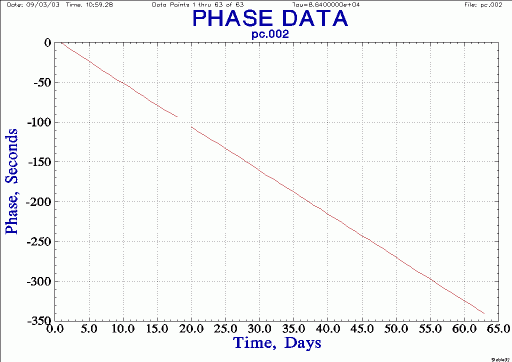
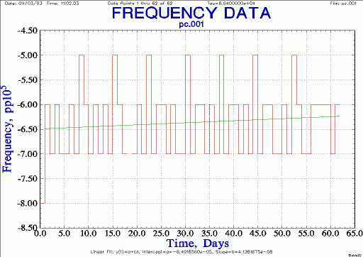
To further pursue this irrelevant tangent let's plot the daily PC time drift data using Stable32.
| PC clock phase, glitch removed |
 |
| PC clock frequency, 1 day resolution |
 |
| PC clock stability |
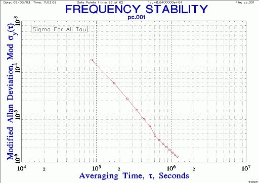 |
So the data logging PC has a frequency error of about -60 ppm, with a drift of about +1 ppm / month. With daily 1 Hz samples, the Allan Deviation of this crystal is on the order of a part in 104th at one day and a part in 106th at two weeks. Note the actual short-term stability is much better than the 1 day points above - but the coarse resolution of the daily snapshot of 1 Hz samples makes the clock look unrealistically bad in this analysis.
Ok, now back to the Rubidium data itself.
With 5 million data points let's use hourly averages instead of the raw 1 Hz data. This data set isn't good for short-term stability analysis anyway (since the Cs reference is not necessarily more stable than the Rb being tested). Also we're mostly interested in drift rate so a tau of one hour is fine.
Stable32 takes forever to read a 100 MB file so we compute averages first:
C:\tvb\rb>avg2 < 523842RH.PHD 86400 > rb-1d
5392237 lines in, 0 lines skipped, 62 lines out, 35437 lines left

C:\tvb\rb>avg2 < 523842RH.PHD  3600 > rb-1h
5392237 lines in, 0 lines skipped, 1497 lines out, 3037 lines left

C:\tvb\rb>avg2 < 523842RH.PHD    60 > rb-1m
5392237 lines in, 0 lines skipped, 89870 lines out, 37 lines left

C:\tvb\rb>wc rb-1d
rb-1d: 0.002 MB, 2 KB, 1922 chars, 124 words, 62 lines

C:\tvb\rb>wc rb-1h
rb-1h: 0.044 MB, 46 KB, 46407 chars, 2994 words, 1497 lines

C:\tvb\rb>wc rb-1m
rb-1m: 2.485 MB, 2546 KB, 2606230 chars, 179740 words, 89870 lines
Using the hourly data set, plot phase (tau is 3600, tag scale is 86400):
| 5065A Rb phase, hourly averages, no editing |
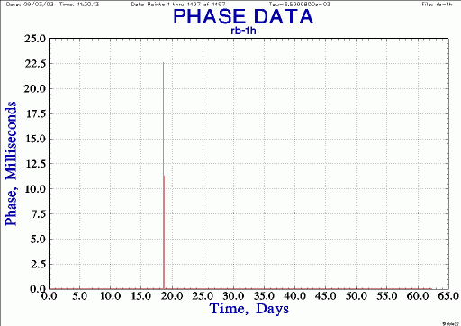 |
Find the obvious data glitch at point 448:
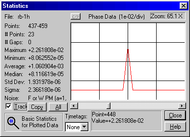
Delete the point and re-plot. As Doug said the first couple of days are warm-up and you can also see a tiny jump near day 18. Let's delete the first 5 days of the run for all further plots.
| 5065A Rb phase, hourly averages, glitch removed |
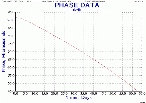 |
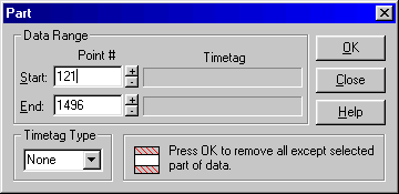
Delete the 5-day (120 hour) warm-up effect:
Convert to frequency and the remaining data glitch is obvious:
| 5065A Rb frequency, no editing |
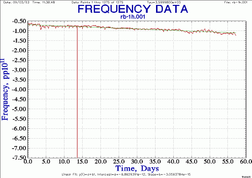 |
Remove frequency glitch:
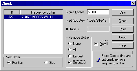
And re-plot. Now we finally have nice looking frequency plot:
| 5065A Rb frequency, hourly averages, glitches removed |
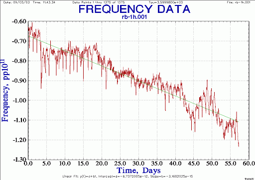 |
The Cs vs. Rb frequency offset is on the order of 1e-11. This seems normal. Now remove the frequency offset and re-plot. This gives a scale that's easier to read (the plot itself is identical to the one above).
Both frequency drift (on the order of 4e-12 over two months) and daily frequency peaks (on the order of 1e-12 per day) are clearly visible:
| 5065A Rb frequency, normalized |
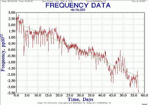 |
Now calculate drift. From experience and independent test we can assume the drift is the result of the 5065A Rb not the 5071A Cs. From the plot above we see a delta f of approximately -4e-12 over two months, or about -2e-12 a month. The actual Stable32 calculation is:
DRIFT FOR FILE: rb-1m.001
Frequency Data Points 1 thru 1377 of 1377
Drift Type: Linear
a=-6.731875e-12
b=-3.171866e-15
c=0.000000e+00
Slope=-3.171866e-15
The calculated frequency drift rate is -3.171866e-15 [per hour] = 7.61e-14 a day = 2.28e-12 per month.
Remove drift and plot one-day frequency averages:
| Rb frequency residuals, daily averages |
Now average to one frequency measurement per day:
Remove drift and look at the offsets:
| Rb frequency residuals, daily averages |
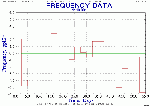 |
How much can we trust this drift value? If one were to calculate drift based on the first 5 days of collecting data the result would be misleading. The same is true if you happened to make a 5-day run starting at day 44 in the above plot. And a 15-day run starting at day 4 would lead you to believe the 5065A has no measurable drift at all!
So what's the correct answer? When calculating monthly drift rates you really need a couple of months of data. And you need to plot the data to make sure there is a believable, relatively smooth, frequency drift line before you use a calculator or computer program to blindly calculate a drift rate.
In this case, I believe two full months of data looks sufficient to conclude that Doug's 5065A drift rate is -2e-12 per month. It is also instructive to see the actual plot and observe that the drift rate changes significantly from day to day or even week to week.
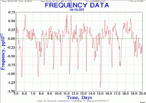
There are spikes on the order of once a day in the two-month frequency plot. Not sure what those are yet; they seem almost too large and too sharp to be temperature related, but they probably are. Note the daily temperature excursions are typically 1e-12 in magnitude which represents the equivalent of two weeks of drift!
Here's a close look at 10 near drift-less days. The frequency excursions are almost always the same time of the day. Given that the data was recorded during Pacific Time (UTC - 8h) the negative frequency peaks appear to correspond to near midnight local time.
| 5065A Rb frequency, showing diurnal peaks |
 |
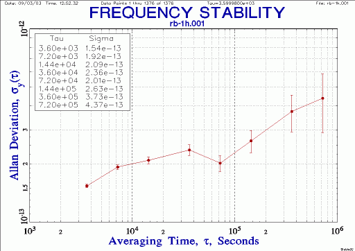
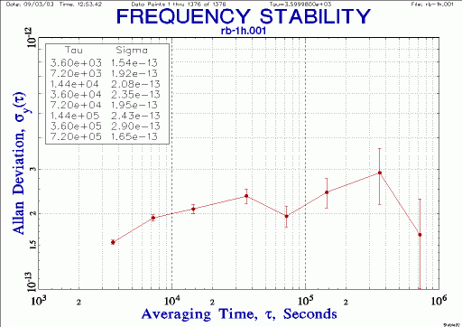
Compare the following plots
1 sec
10 sec
1 min
1 hour
1 day
| 5065A stability |
 |
| 5065A stability, -7.6e-14/day drift removed |
 |
For short-term stability,
C:\tvb\rb>nth < 523842RH.PHD 1 > rb-n1 864000 864000
Window 1
Skip 864000
Take 864000
1728000 lines in, 864000 lines skipped, 864000 lines out
asdfasdf
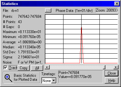
Cs not necessarily the best reference
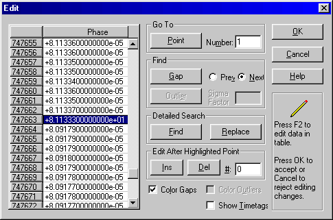
Ignore time stamps, assume 1 Hz, pick 10 day
Take the best 10 day segment of the data.
Delete (one phase jump) two frequency jumps and Fill.
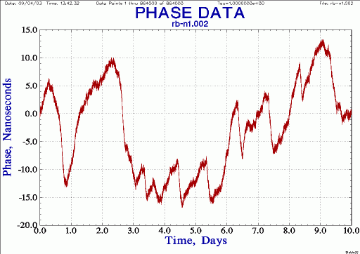
Near drift-less. Only diurnal effects.
Extract 10 days from data set.
Bump up Stable32 max data count.
Prune, fill
7 days (avoid data glitch)
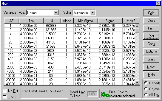
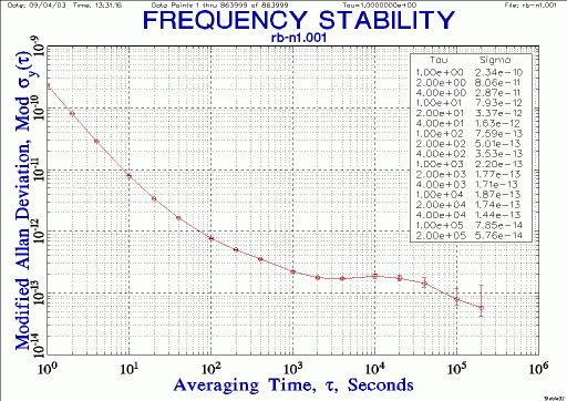
T.I. counter is 5370B. So most of the noise below an hour is measurement noise.
| Best 10 days: 5065A vs. 5071A stability - from 1 to 100k seconds |
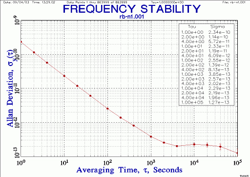 |
Here's the same but using MDEV instead of ADEV:
| Best 10 days: 5065A vs. 5071A stability - MDEV |
 |
| Best 10 days: phase |
 |
DRIFT FOR FILE: rb-n10
Frequency Data Points 1 thru 513304 of 513304
Drift Type: Quadratic
a=9.103293e-05
b=-6.753136e-11
c=-4.044817e-17
Slope=-8.089634e-18